How to Freeze and Unfreeze Panes in Excel

How to Freeze and Unfreeze Panes in Excel

Freezing Panes allow you to keep an area of an Excel sheet visible while you scroll through the rows and columns, this is useful as it makes the excel sheets easier to read.

Freezing panes

To Freeze panes on an Excel sheet:

• Click on the “View” tab
• Click on “Freeze Panes”

You will now be greeted with a few options.

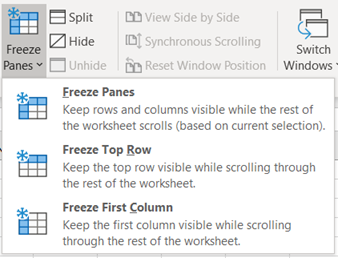
The second and third options in the screenshot above are self-explanatory and will freeze either the first row or column based on which you select. However, option one allows you more freedom.

For example, if you wish to freeze the first three rows in an excel file, you would select the entire fourth row and then click the “Freeze Panes” to freeze all rows above.

If you wish to freeze columns as well as rows, you would need to select the cell below the rows and to the right of the columns you want to keep visible when you scroll.

Unfreezing panes

You may find that some Excel sheets have too many frozen panes and limit the amount of data that you can view on screen. If you run into this, or you have accidentally frozen too many panes, you can unfreeze the panes.

To unfreeze panes on an Excel sheet:

• Click on the “View” tab
• Click on “Freeze Panes”
• Click on “Unfreeze Panes”

You should now be able to scroll freely through the file